6. DAT for Python
6.1. Overview
The main objective of the Data Analytics Toolkit is to facilitate the exploitation of the multi-variate data set in the ESDC for experienced users and empower less experienced users to explore the wealth of information contained in the ESDC. To this end, Python is almost a natural choice for the programming language, as it is easy to learn and use, offers numerous, well-maintained community packages for data handling and analysis, statistics, and visualisation.
The DAT for Python relies primarily on xarray a package that provides N-dimensional data structures and efficient computing methods on those object. In fact, xarray closely follows the approach adopted NetCDF, the quasi-standard file format for geophysical data, and provides methods for many commonly executed operations on spatial data. The central data structure used for representing the ESDC in Python is thus the xarray.Dataset.
Such dataset objects are what you get when accessing the cube’s data as follows:
from cablab import Cube
cube = Cube.open("/home/doe/esdc/cablab-datacube-0.2.4/low-res")
dataset = cube.data.dataset(["precipitation", "evaporation", "ozone", "soil_moisture","air_temperature_2m"])
Any geo-physical variable in the ESDC is represented by a xarray.DataArray, which are Numpy-like data arrays with additional coordinate information and metadata.
The following links point into the xarray documentation, they provide the low-level interface for the Python DAT:
- Indexing and selecting data
- Computation
- Split-apply-combine
- Reshaping and reorganizing data
- Combining data
- Time series data
Building on top of the xarray API the DAT offers high-level functions for ESDC-specific workflows in the cablab.dat module. These functions are addressing specific user requirements and the scope of the module will increase with the users of the DAT. In the following, typical use cases and examples provide an illustrative introduction into the usage of the DAT and thus into the exploration of the ESDC.
6.2. Use Cases and Examples
The below examples are all contained in a Jupyter notebook, which is also available in the E-Lab.
6.2.1. Data Access and Indexing
In the first step described above, a subset of five variables is loaded into the DataSet, which distinguishes between Dimensions, Coordinated, and Data Variables, just like NetCDF.
dataset
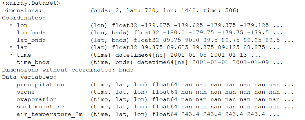
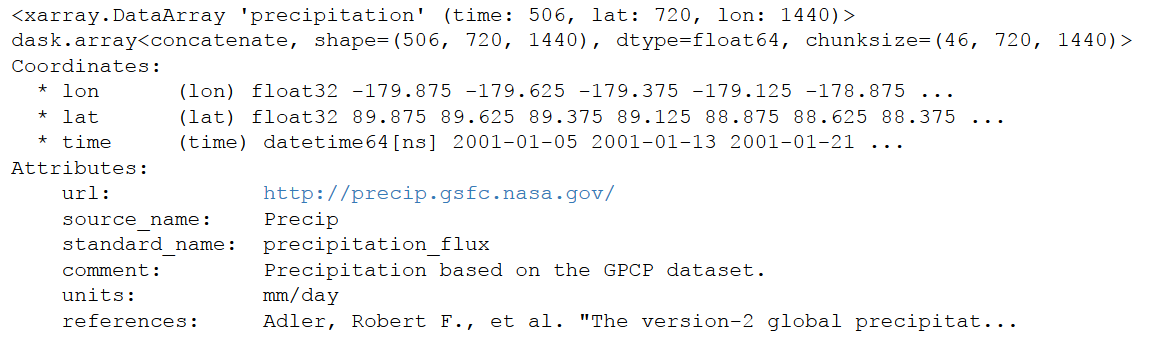
Addressing a single variable returns a xarray DataArray and reveals the metadata associated to the variable. Note the similarity to the Pandas syntax here.
dataset.precipitation
The actual data in a variable can be retrieved by calling dataset.precipitation.values, which returns a
numpy array.
isinstance (dataset.precipitation.values,np.ndarray)

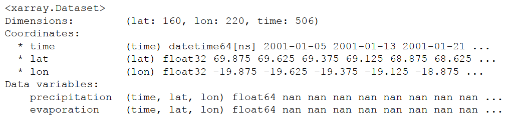
xarray offers different ways for indexing, both integer and label-based look-ups, and the reader is referred to the exhaustive section in the respective section of the xarray documentation: xarray Indexing and selecting data. The following example, in which a chunk is cut out from the larger data set, demonstrates the convenience of xarrays syntax. The result is again a xarray DataArray, but with only subset of variables and restricted to a smaller domain in latitude and longitude.
dataset[['precipitation', 'evaporation']].sel(lat = slice(70.,30.), lon = slice(-20.,35.))
6.2.2. Computation
It was a major objective of the Python DAT to facilitate processing and analysis of big, multivariate geophysical data sets like the ESDC. Typical use cases include the execution of functions on all data in the ESDC, the aggregation of data along a common axis, or analysing the relation between different variables in the data set. The following examples shed a light on the capabilities of the DAT, more typical examples can be found in the Jupyter notebook and the documentation of xarray provides an exhaustive reference to the package’s functionalities.
Many generic mathematical functions are implemented for DataSets and DataArrays. For example, an average over all variables in the dataset can thus be easily calculated.
dataset.mean(skipna=True)
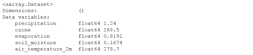
Note that calculating a simple average on a big data set
may require more resources, particularly memory, than is available on the machine you are working at. In such cases,
xarray automatically involves a package called dask for out-of-core computations and automatic parallelisation. Make
sure that dask is installed to significantly improve the user experience with the DAT. Similar to pandas, several
computation methods like groupby or apply have been implemented for DataSets and DataArrays. In
combination with the datetime data types, a monthly mean of a variable can be calculated as follows:
dataset.air_temperature_2m.groupby('time.month').mean(dim='time')
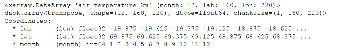
In the resulting DataArray, a new dimension month has been automatically introduced.
Users may also define their own functions and apply them to the data. In the below example, zcores are computed for
the entire DataSet by usig the built-in functions mean and std. The user function
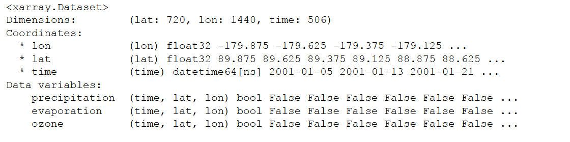
above_Nsigma is applied to all data to test if a zscore is above or below two sigma, i.e. is an outlier. The
result is again a DataSet with boolean variables.
def above_Nsigma(x,Nsigma):
    return xr.ufuncs.fabs(x)>Nsigma

zscores = (dataset-dataset.mean(dim='time'))/dataset.std(dim='time')
res = zscores.apply(above_Nsigma,Nsigma = 2)
res
In addition to the functions and methods xarray is providing, we have begun to develop high-level functions that
simplify typical operations on the ESDC. The function corrcf computes the correlation coefficient between
two variables.
6.2.3. Plotting
Plotting is key for the explorative analysis of data and for the presentation of results. This is of course even more so for Earth System Data. Python offers many powerful approaches to meet the diverse visualisation needs of different use cases. Most of them can be used with the ESDC since the data can be easily transferred to numpy arrays or pandas data frames. The following examples may provide a good starting point for developing more specific plots.
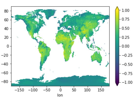
Calculating the correlation coefficient of two variables and plot the resulting 2D image af latitude and longitude.
cv = DAT_corr(dataset, 'precipitation', 'evaporation')
cv.plot.imshow(vmin = -1., vmax = 1.)
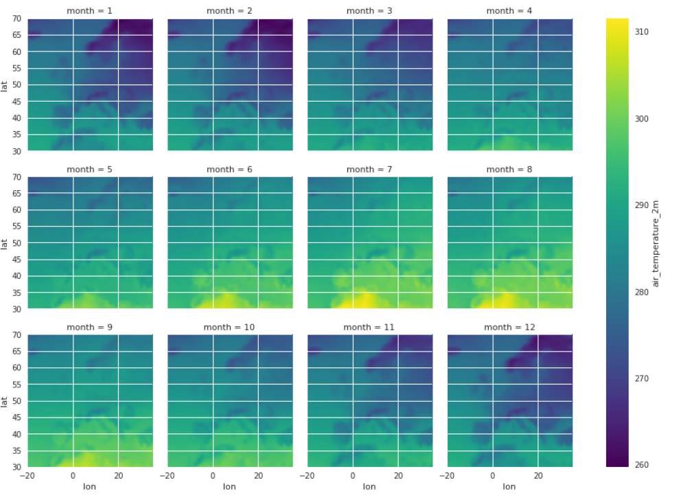
Plotting monthly air temperature in twelve subplots.
Air_temp_monthly = dataset.air_temperature_2m.groupby('time.month').mean(dim='time')
Air_temp_monthly.plot.imshow(x='lon',y='lat',col='month',col_wrap=3)
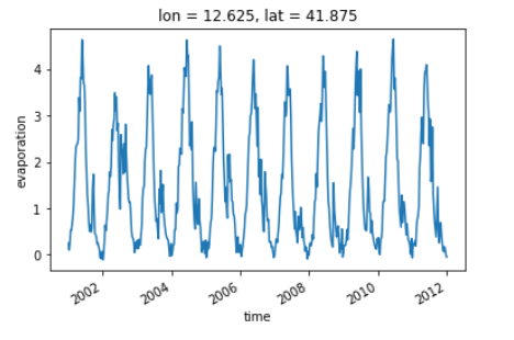
A simple time-series plot at a given location.
dataset.evaporation.sel(lon = 12.67,lat = 41.83, method = 'nearest').plot()
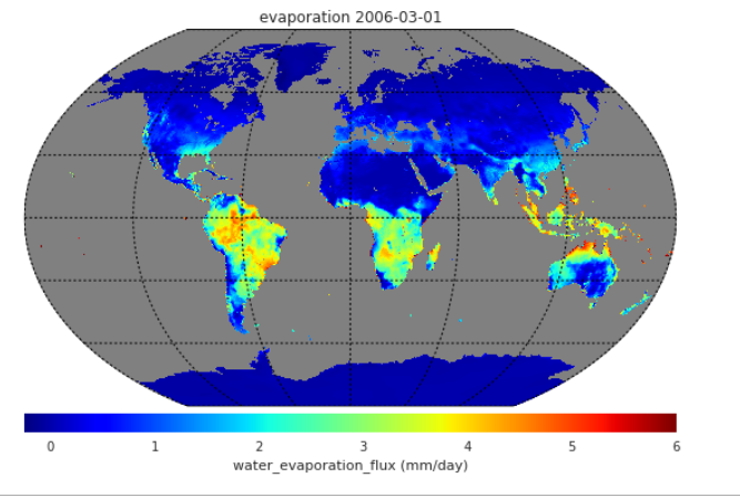
Plotting a projected map using the DAT function map_plot.
.. code-block:: python
fig, ax, m = map_plot(dataset,’evaporation’,‘2006-03-01’,vmax = 6.)
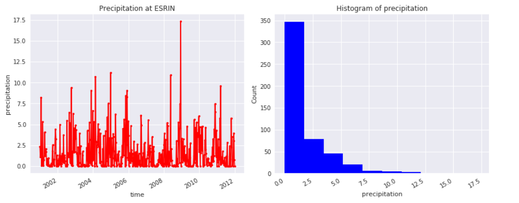
Generating a subplot of a time-series at a given location and the associated histogram of the data.
precip1d = dataset['precipitation'].sel(lon = 12.67,lat = 41.83, method = 'nearest')
fig, ax = plt.subplots(figsize = [12,5], ncols=2)
precip1d.plot(ax = ax[0], color ='red', marker ='.')
ax[0].set_title("Precipitation at ESRIN")
precip1d.plot.hist(ax = ax[1], color ='blue')
ax[1].set_xlabel("precipitation")
plt.tight_layout()
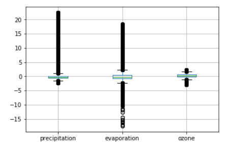
Convert a DataSet into an pandas dataframe and generate a boxplot from the dataset.
zscore = (dataset-dataset.mean(dim='time'))/dataset.std(dim='time')
df = zscore.to_dataframe()
df.boxplot(column=["precipitation","evaporation","ozone"])
6.3. Python API Reference
The low-level interface of the ESDC Python DAT is the xarray API.
The following functions provide the high-level API of the ESDC Python DAT:
The following functions provide the high-level API of the ESDC Python DAT. It provides additional analytical utility functions which work for xarray.Dataset objects which are used to represent the ESDC data.
-
cablab.dat.corrcf(ds, var1=None, var2=None, dim='time')[source]¶ Function calculating the correlation coefficient of two variables var1 and var2 in one xarray.Dataset ds.
Parameters: - ds – an xarray.Dataset
- var1 – Variable 1
- var2 – Variable 2, both have to be of identical size
- dim – dimension for aggregation, default is time. In the default case, the result is an image
Returns:
-
cablab.dat.map_plot(ds, var=None, time=0, title_str='No title', projection='kav7', lon_0=0, resolution=None, **kwargs)[source]¶ Function plotting a projected map for a variable var in xarray.Dataset ds.
Parameters: - ds – an xarray.Dataset
- var – variable to plot
- time – time step or datetime date to plot
- title_str – Title string
- projection – for Basemap
- lon_0 – longitude 0 for central
- resolution – resolution for Basemap object
- kwargs – Any other kwargs accepted by the pcolormap function of Basemap
Returns: